[SQUEAKING]
[RUSTLING]
[CLICKING]
VASILY STRELA: The rest of the class, let’s talk a little bit about interest rates and a little bit about bonds, because that’s very important and central for many-- will be definitely part of many classes and is generally central for finance, and for life, in my opinion.
So what is interest? Well, let’s start with now. And suppose we have $1 which we invested-- well, put it in the bank. So what happens in one year? Well, you expect to get your dollar back with some interest. And what does it mean? So you get 1 plus something. I don’t know-- 5% nowadays. And this r is called interest rate.
So what happens if you reinvest it. What will you get? The whole thing. So in two years you would expect to get 1 plus r times 1 plus r. So 1 plus r squared. So in n years, you will expect to get 1 plus r to the power n.
Well, let’s make it small and small not to confuse ourselves. So now let’s make life a little bit more complicated. What happens if you decide to take your money in half a year? You had one here.
So what happens in half a year? Well, you get half of the interest. So it will be 1 plus r over 2. And in one year, it will be 1 plus r over 2 squared because you reinvest it. So suppose you keep it in the bank. And in n years, it will be 1 plus r over 2 but twice n. Because there are twice as many periods
Let’s subdivide further. Let’s make m period. So in the first period, you get 1 over-- 1 plus r over m. In one year, it will be 1 plus r over m to the power m. And here, you’ll get 1 plus r over m-- m times m.
What if we take the limit. If we are able to reinvest every second, every millisecond, what happens then? So we’ll send this m to the infinity. So what is-- who knows what is that?
AUDIENCE: e.
VASILY Well, it is e, but–
STRELA:
AUDIENCE: r.
VASILY r.
STRELA:
VASILY STRELA:
AUDIENCE: Oh, sorry. r.
Right. r has to be there, and this n will stay there. Well, yeah. Yeah, if we keep m here. So in fact, interesting historical fact, that’s how e was discovered and defined. It was Bernoulli in his seminal paper in 1683, where he described this computation. And it was about interest rates, about how interest is compounding. So maybe this was the first mathematical finance paper in the history.
Now, let’s change the game a little bit-- not the game-- change the question a little bit. So suppose we know that we will receive $1 in one year. How much should we pay for this right to receive $1 in one year? How much should we pay now to receive $1 in one year? And let’s compute it.
So suppose we don’t know. Let’s assume that now it is x dollars. And let’s consider the following strategy. Let’s borrow $1-- let’s borrow x, this amount now, and let’s see what happens at the end.
So at the end, in one year, I mean, we’ll receive $1 for sure. And we’ll have to repay our debt but with interest. So we’ll have repay 1 plus x times r. Sorry-- x times 1 plus.
Now, what should this be? Can it be greater than zero, this difference? Well, if it’s greater than zero, why wouldn’t we borrow-- why wouldn’t we buy a right to receive a billion dollars, then we’ll have a lot of profit?
Can it be less than zero? Well, then we would be stupid to enter this contract because we’ll lose money for sure. We know that this will happen in one year. So for no arbitrage– and we don’t assume that our counterparty is stupid. We don’t think that we are stupid. So it has to be zero.
And this x is equal to 1 plus-- divided by 1 plus r. And this is called discounting, meaning that if we know that we’ll receive a certain amount in the future, and we know the interest rates, prevailing interest rates, then we have to discount the future value to today using a discount factor. And this is the discount factor assuming annualized compounding.
If we assume annualized compounding and receive n dollars in the future, in the future n years, the value of n dollars in the future, it is the value of our n dollars, which we are receiving in the future n years, but it has to be discounted by n years. So it should be–
And here, it is discounting. If we assume a continuous discounting, something like this, then it will be-- our price will be n times e to the minus rn. This will be our discount factor, assuming continuous compounding. And we already hitting the problem-- or not the problem. But we are already hitting a situation where some model is needed, which brings us to the world of financial instruments-- interest rate related financial instruments.
And the simplest financial instrument is a zero-coupon bond. That’s exactly the right to receive certain amount of notional. Or notional-- or quite often 1 or 100 in certain amount of time. And that’s the value of our zero-coupon bond.
More common financial instruments are coupon bonds. Because most people would like to receive periodic interest for lending money. And that’s effectively lending money. And this is typical bonds. For example, if you buy government bonds that’s what will happen. You’ll give the government your $100, and government will be repaying you coupons periodically, usually semiannually, here in the US-- in Europe, it’s quite often quarterly- and the notional, all your $100, at the end.
So what the price of such a coupon bond should be? Well, we’ll need to take all the cash flows and discount them. And if we assume a constant interest rate, we’ll have to discount it with our constant discount factors. And that’s how much-- and this assumes-- well, say annual coupons and annual rate. So that will be your sequence with a notional at the end, the whole big notional at the end.
And can we sum this up? Well, sure. That’s geometric sequence. Everybody can sum up geometric sequence. And that’s the value. That’s what you get. And that’s the value of the bond.
Now, the bonds are traded on the markets. There are prices of the bonds. And if you start investing into bonds, and not in just in one bond, you should be able to compare to bonds. And comparing the price is not really convenient because bonds have different maturities. Even with the same interest, would have different prices because there will be different number of cash flows. Bonds of different coupons will have different prices.
So what turns out to be more convenient measure to compare bonds and various fixed income securities is yield. And yield is such a constant interest rate, which by this discounting gives you market price. So you buy something at the market price. You know the market price. So all the cash flows. So you back out one flat interest rate, which will give you the price of the bond. That’s called yield of the bond.
Obviously, there is one-to-one relationship between price and yield. So for our zero-coupon bond, yield is pretty simple. You just invert this formula. And this is here on the slide. For coupon bonds, yield computation is more complex because inverting this formula is more involved. And in fact, it has to be numerical. But that’s how yields are computed.
Here, I’ll I give you an example of a few-- of price yield relationship for a 10-year bond with different coupons. So what’s important to know here is that the higher the coupon-- and that’s natural-- the higher the yield is for the same bond of the same maturity. But what is important to know is the yield and price are in inverse relationship. The high yield, the lower the price because it’s all about discounting. It’s in the denominator. The higher the price, the lower the yield.
So that’s what it is. But real life is more complicated than that. In real world, as if we wanted everything to be the same simple interest rate, and all bonds have to be discounted the same, real life is slightly different.
So if you take markets-- securities, market bonds and start breaking up their yields, they will not be constant, particularly with maturity. And this is called the yield curve. And I gave you-- here, I plotted a yield curve for a 10-year-- term structure of 10-year yields, US government yields, for a variety of times. And I want to talk just a little bit about it because it’s quite topical.
So that’s the thickest line is this. That’s the yield curve for September 3, so two days ago. So quite different. And yields here for a very short-dated securities are quite higher than for long-dated securities. This is still quite atypical.
For example, in '92, around the same September time, yield curve looked like this-- considered to be more or less classical curve. And generally speaking, we expect upward-sloping curves because generally speaking, people would like to receive more yield for a longer term investments.
And that’s what was the case in-- this is what-- this is '21. This is '14. Yeah, nice looking curves. The only difference here is that now they are-- in '92, they were grounded at 3% and went all the way up to 7%, those were grounded at zero and went only to 2%, 3%.
Now, interesting observation here is-- let’s look at this inverted curves. A year ago it was inverted. Now it is inverted. It was inverted in 2007. No, this is 2019, and this is 2007. So what the-- do we have anything in your mind what’s common between 2021 and 2007? So–
AUDIENCE: The year before the recession.
VASILY STRELA: Yes, exactly. Well, 2007, the recession was “The Recession.” 2021-- there was a recession in 2020. Even this yield curve is before COVID. So nothing was–
And if you look at the shape of the yield curves and recession times, well, it is common analogy-- and there are papers on that-- how predictive is inverted yield curve for the recessions? Generally, it is assumed to be predictive. So here we go. We have an inverted yield curve. What does it tell us about the future?
Well, that’s all Fed’s job to keep it-- to make it a soft landing and for a recession not to happen. And we’ll see. Maybe it will be, or maybe not.
But what I want to emphasize that there is a lot of information in yield curves. One of the lectures in the future, Andrew Gunstensen, he will be talking mostly about yield curves and yield curve constructions and the instruments around that. So it’s very important piece of knowledge.
And yeah, I’ll promise you, when I come back later on to talk about Black-Scholes, I’ll bring this slide back, and we’ll see what happens with the yield curve. Because what-- and I can guarantee you it will look different because the Fed is happening-- the Fed meeting is happening in September. Everybody expects the yields to be cut, which immediately will bring the short end down. What happens with the long end? I wish I knew. Anyway, that’s about yield curves.
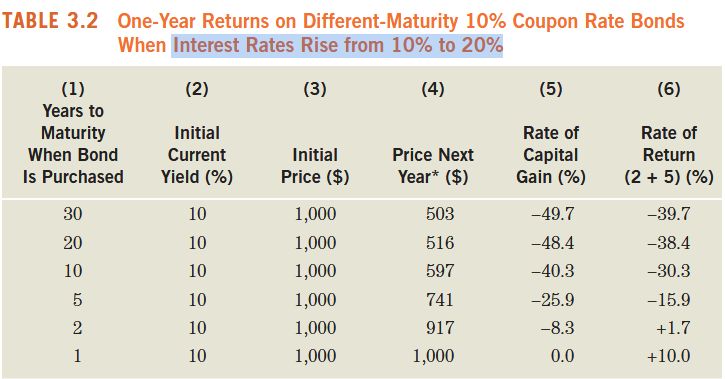
But another important thing to emphasize that no matter what, bond prices are sensitive to yields, obviously. And they are sensitive to yields in nonlinear fashion. What does it mean? Well, it means that if you hold bonds on your hands and yields change, and they do change, your investment will change. So it’s quite important to understand the sensitivity of your investment to interest rates and yields.
And what are sensitivities? Those are derivatives. Or in finance and fixed income world, they’re called durations because they’re usually scaled by price. So very important measures are duration of the bond, which is derivative with respect to yield. And for each different bond and each different security, they will be slightly different.
And not only the first derivative is important, the second derivative or convexity is also important. So yeah. And that’s what we’ll be talking about in various classes.
We will be talking about more interesting interest rate objects in the future, in particular, forward rates and swaps. But I’ll leave it to Stefan and Andrew to talk more about that. That’s probably all for today. And any questions to any of us?
AUDIENCE: Have you done this-- have you done that game before?
SPEAKER: Not specifically in this format. So we tried-- before it was more open-ended. I was thinking-- so I think by fixing the dates, you don’t have to make the market timing decision. We already made it for you. Yeah
mit18_642_f24_lec01_1.pdf (522.2 KB)